Atmospheric Drag Model | Essay

The atmospheric drag

1 – Introduction

The principal non-gravitational force acting on satellites in Low-Earth Orbit (LEO) is atmospheric drag. This effect for a LEO satellite has direct implications in satellite lifetime. Indeed, drag acts in the opposite direction of the velocity vector and removes energy from the orbit. This energy reduction causes to the orbit to get smaller, leading to further increases in drag. Eventually, the altitude of the orbit becomes so small that the satellite reenters in the atmosphere.

What Citation Styles Can You Use for My Essay?

Students often ask, “Can you write my essay in APA or MLA?”—and the answer’s a big yes! Our writers are experts in every style imaginable: APA, MLA, Chicago, Harvard, you name it. Just tell us what you need, and we’ll deliver a perfectly formatted paper that matches your requirements, hassle-free.

The equation for acceleration due to drag is:

• : atmospheric density (kg.m^-3)
• satellite’s cross-sectional area (m²)
• : satellite’s mass (kg)
• : satellite’s velocity with respect to the atmosphere (m.s^-2)
• : drag coefficient (dimensionless)
• : ballistic coefficient

Drag presents a challenge to accurate modeling, because the dynamics of the upper atmosphere are not completely understood, in part due to the limited knowledge of the interaction of the solar wind and the Earth’s magnetic field. In addition, drag models contain many parameters that are difficult to estimate with reasonable accuracy: atmospheric density, ballistic coefficient, cross-sectional area… Calculating atmospheric density is often the most difficult part of assessment in modeling the atmosphere. Its complexity is apparent from the sheer number of regime. In addition, although values are shown for temperature and altitude, they all change over time and are very difficult to predict.

Strong drag occurs in dense atmospheres, and satellites with perigees below 120 km have such short lifetimes that their orbits have no practical importance. Above 600 km, on the other hand, drag is so weak that orbits “usually” last more than the satellites’ operational lifetimes. At this altitude, perturbations in orbital period are so slight that we can easily account for them without accurate knowledge of the atmosphere density. At intermediate altitudes however, roughly two variable energy sources cause large variations in atmospheric density and generate orbital perturbations: the geomagnetic field and solar activity. These variations can be predicted with two empirical models: the Mass Spectrometer Incoherent Scatter (MSIS) and the Jacchia models.

Is It Legal to Use Your Writing Service?

Absolutely, it’s 100% legal! Our service provides sample essays and papers to guide your own work—think of it as a study tool. Used responsibly, it’s a legit way to improve your skills, understand tough topics, and boost your grades, all while staying within academic rules.

Knowing that the considered satellite should be at an altitude of 700 km (the last launches of nano-satellites demonstrate that the start altitude is often very inaccurate), the Jacchia model is the most accurate one to estimate atmospheric density, and in this way satellite lifetime.

2 – The Jacchia atmospheric density model

The Jacchia atmospheric density model formulation is very common, but also very complex. The model contains analytical expressions for determining exospheric temperature as a function of position, time, solar activity and geomagnetic activity. With a computed temperature, density can be calculated from empirically determined temperature profiles or from the diffusion equation. Then the overall approach is to model the atmospheric temperature.

In this way, to simplify the analytical resolution, the altitude range will be constraint from the start altitude at 700 km to 200 km.

How Much Does It Cost to Get a Paper Written?

Our pricing starts at $10 per page for undergrad work, $16 for bachelor-level, and $21 for advanced stuff. Urgency and extras like top writers or plagiarism reports tweak the cost—deadlines range from 14 days to 3 hours. Order early for the best rates, and enjoy discounts on big orders: 5% off over $500, 10% over $1,000!

1 > Evaluating temperature

Jacchia defines the region above 125 km in altitude with an empirical, asymptotic function for temperature:

• : distance between satellite and ground station (“height above the reference ellipsoid”) (km)
• : base value temperature (Kelvin)
• : corrected exospheric temperature (Kelvin)

• : inflection point temperature (Kelvin)

As needed in the two equations above, the corrected exospheric temperature is defined as below:

• : uncorrected exospheric temperature (Kelvin)
• : correction factor for exospheric temperature (Kelvin)

represents the exospheric temperature without any correction. It is based on the nighttime global exospheric temperature, excluding all effects of geomagnetic activity:

Do You Use AI to Write Papers?

No way—our papers are 100% human-crafted. Our writers are real pros with degrees, bringing creativity and expertise AI can’t match. Every piece is original, checked for plagiarism, and tailored to your needs by a skilled human, not a machine.

Where is the average daily solar flux at a 10.7 cm wavelength for the day of interest and is an 81-day running average of values, centered on the day of interest. Because the effect of solar flux on atmospheric density lags one day behind the observed values, calculations can (at best) use values which are one day old. The resulting value of can be used now to determine the uncorrected exospheric temperature.

• 
• 
• : sun’s declination
• : geodetic latitude of the satellite
• , (-180° < < 180°)

Actually can be determined from the dot product and the two vectors for the Sun and the satellite. More complicated methods are available to determine the, but the precision here does not need extra accuracy.

Why Choose You for Research Papers?

We’re the best because our writers are degree-holding experts—Bachelor’s to Ph.D.—who nail any topic. We obsess over quality, using tools to ensure perfection, and offer free revisions to guarantee you’re thrilled with the result, even on tight deadlines.

Now the geomagnetic activity and its effect on temperature have to be corrected. The correction factor for exospheric temperature,, depends on the geomagnetic index, , and is calculated for altitudes at least 200 km. The actual value of is with a 3-hour lag, in which the molecular intersection build up and the change in density would be noticed.

2 > Evaluating density scale height

For planetary atmospheres, density scale height describes a difference in height, over which the density of the atmosphere changes significantly by a factor e (approximately 2.71828 , the base of natural logarithms, decreasing upward). Usually, the scale height remains constant for a particular temperature. However, in the upper part of the atmosphere, it changes significantly and in different ways. For instance, at heights over 100 km, molecular diffusion means each molecular atomic species has it own scale height. This part will only focus on density scale height at altitude above 105 km.

Who’s Writing My College Essays?

Our writers are top-tier—university grads, many with Master’s degrees, who’ve passed tough tests to join us. They’re ready for any essay, working with you to hit your deadlines and grading standards with ease and professionalism.

The temperature profile has to be integrated in the total number density of the five atmospheric components, in order to achieve their individual effect on the standard density. As the altitude assumed above 500 km, the concentration of hydrogen have to be taken into account also. First of all, the hydrogen number density at 500 km altitude (in cm^-3):

Implemented in the hydrogen number density equation for altitude greater than 500 km:

• : molecular mass of hydrogen
• erg/°K : Boltzmann’s constant

Then the number density of the other atmospheric components which are nitrogen N₂, oxygen molecular O₂ and atomic O, and helium He (in cm^-3):

• i denotes N2, O2, O or He
• : number density of each constituent at 105 km altitude
• : thermal diffusion coefficient (only for Helium)

The correction for Helium number density because of seasonal-latitudinal variations is (dimensionless):

And implemented here:

Finally, the total number density is given by (in cm^-3):

Hence, the mass density (in gm/cm^-3):

• : mass of the constituent I in gm/mole
• 
• 
• 
• 
• 

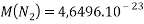
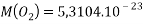
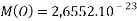
Which gives the molecular mass:

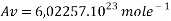• : Avogadro’s number

Finally, the density scale height, according to the temperature profile which depends mainly of the satellite’s altitude and position from the Sun:

• : universal gas constant

3 > Evaluating density

Jacchia used a standard exponential relation to evaluate density:

• : base atmospheric density (kg.m^-3)
• : distance between satellite and ground station (“height above the reference ellipsoid”) (km)
• : base altitude (km)
• : scale height (km)

An interesting point to highlight is below 150 km, the density is not strongly affected by solar activity. However, at satellite altitudes in the range of 500 to 800 km, the density variations between solar maximum and solar minimum are approximately 2 orders of magnitude. The large variations in density imply that satellites will decay more rapidly during periods of solar maxima and much more slowly during solar minima. The effect of the solar maxima will also depend on the satellite ballistic coefficient. Those with a low ballistic coefficient will respond quickly to the atmosphere and will tend to decay promptly. Those with high ballistic coefficients will push through a larger number of solar cycles and will decay much more slowly. Note that time for satellite decay is generally measured better in solar cycles than in years. From there to lifetimes of about half a solar cycle (approximately 5 years) there will be a very strong difference between satellites launched at the start of a solar minimum and those launched at the start of solar maximum.

The first correction to apply to this equation is for seasonal latitudinal variation in the lower thermosphere:

• : geodetic latitude, measured positively north from the equator (deg)
• : Julian date of 1958 (years)

The Julian date of 1958 is used to determine the number of years from 1958. is the number of days from January 1, 1958:

The correction for semi-annual variations is as below:

This correction uses an intermediate value :

For altitudes above 200 km, the geomagnetic effect can be neglected on density. Hence, these corrections can be apply to the standard density:

Giving the final corrected density:

Even though any model cannot do a real adequate job of modeling the atmosphere, the Jacchia model continues to perform exceptionally well compared to the others and is the fastest overall. Moreover, it is the only one which give analytical formulas which can be computed without external values, even though that degrades the result in a way.

3 – The ballistic coefficient

Drag also depends on the ballistic coefficient, defined as a body measure of the ability to overcome air resistance in flight. For instance, satellites in LEO with high ballistic coefficients experience smaller perturbations to their orbits due to atmospheric drag. In regards to the nano-satellite analysis, mass and cross-sectional area do not change at any time. Actually, nano-satellite cannot change their position because they do not have any ergol propellers. Hence this coefficient depends mainly of the drag one.

The drag coefficient of any object comprises the effects of the two basis contributors to fluid dynamic drag: skin friction and form drag. In most cases, this coefficient is estimated. Considering the configuration of the spacecraft as a regular brick-like shape and the environment conditions, it is estimated here at 2,1. Theoretically, it is highly impossible to have an exact solution, only experiments might approximate it.

Tags: 1500 Words Assessment Task, Ace Homework Tutors, Assignment Homework Help & Answers, Create a 2-4 page resource